From Wikipedia, the free encyclopedia
A price index (plural: “price indices” or “price indexes”) is a normalized average (typically a weighted average) of price relatives for a given class of goods or services in a given region, during a given interval of time. It is a statistic designed to help to compare how these price relatives, taken as a whole, differ between time periods or geographical locations.
Price indexes have several potential uses. For particularly broad indices, the index can be said to measure the economy's price level or a cost of living. More narrow price indices can help producers with business plans and pricing. Sometimes, they can be useful in helping to guide investment.
Some notable price indices include:
![]()
 William Fleetwood
While Vaughan can be considered a forerunner of price index research, his analysis did not actually involve calculating an index.[1] In 1707 Englishman William Fleetwood created perhaps the first true price index. An Oxford student asked Fleetwood to help show how prices had changed. The student stood to lose his fellowship since a fifteenth-century stipulation barred students with annual incomes over five pounds from receiving a fellowship. Fleetwood, who already had an interest in price change, had collected a large amount of price data going back hundreds of years. Fleetwood proposed an index consisting of averaged price relatives and used his methods to show that the value of five pounds had changed greatly over the course of 260 years. He argued on behalf of the Oxford students and published his findings anonymously in a volume entitled Chronicon Preciosum.[2]
William Fleetwood
While Vaughan can be considered a forerunner of price index research, his analysis did not actually involve calculating an index.[1] In 1707 Englishman William Fleetwood created perhaps the first true price index. An Oxford student asked Fleetwood to help show how prices had changed. The student stood to lose his fellowship since a fifteenth-century stipulation barred students with annual incomes over five pounds from receiving a fellowship. Fleetwood, who already had an interest in price change, had collected a large amount of price data going back hundreds of years. Fleetwood proposed an index consisting of averaged price relatives and used his methods to show that the value of five pounds had changed greatly over the course of 260 years. He argued on behalf of the Oxford students and published his findings anonymously in a volume entitled Chronicon Preciosum.[2]
 of goods and services, the total market value of transactions in in some period
  would be
 and
and  , the same quantities of each good or service were sold, but under different prices, then
Of course, for any practical purpose, quantities purchased are rarely if ever identical across any two periods. As such, this is not a very practical index formula.
One might be tempted to modify the formula slightly to
and while quantities stay the same:  will double. Now consider what happens if all the quantities double between and while all the prices stay the same: will double. In either case the change in is identical. As such, is as much a quantity index as it is a price index.
Various indices have been constructed in an attempt to compensate for this difficulty.
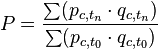
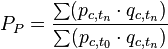
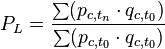
The Paasche index is computed as
is the relative index of the price levels in two periods, is the base period (usually the first year), and the period for which the index is computed.
Note that the only difference in the formulas is that the former uses period n quantities, whereas the latter uses base period (period 0) quantities.
When applied to bundles of individual consumers, a Laspeyres index of 1 would state that an agent in the current period can afford to buy the same bundle as she consumed in the previous period, given that income has not changed; a Paasche index of 1 would state that an agent could have consumed the same bundle in the base period as she is consuming in the current period, given that income has not changed.
Hence, one may think of the Paasche index as one where the numeraire is the bundle of goods using current year prices and current year quantities. Similarly, the Laspeyres index can be thought of as a price index taking the bundle of goods using current prices and base period quantities as the numeraire.
The Laspeyres index tends to overstate inflation (in a cost of living framework), while the Paasche index tends to understate it, because the indices do not account for the fact that consumers typically react to price changes by changing the quantities that they buy. For example, if prices go up for good then, ceteris paribus, quantities of that good should go down.
 and
and  :
:
However, there is no guarantee with either the Marshall–Edgeworth index or the Fisher index that the overstatement and understatement will exactly cancel the other.
While these indices were introduced to provide overall measurement of relative prices, there is ultimately no way of measuring the imperfections of any of these indices (Paasche, Laspeyres, Fisher, or Marshall–Edgeworth) against reality.[citation needed]
In practice, price indexes regularly compiled and released by national statistical agencies are of the Laspeyres type, due to the above mentioned difficulties in obtaining current-period quantity or expenditure data.
Here is a reformulation for the Laspeyres index:
Let be the total expenditure on good c in the base period, then (by definition) we have
  and therefore also
  . We can substitute these values into our Laspeyres formula as follows:
is the period for which we wish to calculate the index and is a reference period that anchors the value of the series:
 and period ". When you multiply these all together, you get the answer to the question "by what factor have prices increased since period ".
Nonetheless, note that, when chain indices are in use, the numbers cannot be said to be "in period" prices.
 , where
  and
and  are vectors giving prices for a base period and a reference period while
  and
and  give quantities for these periods.[5]
The problem discussed above can be represented as attempting to bridge the gap between the price for the old item at time t, , with the price of the new item at the later time period,
  .[7]
.[7]
Price indexes have several potential uses. For particularly broad indices, the index can be said to measure the economy's price level or a cost of living. More narrow price indices can help producers with business plans and pricing. Sometimes, they can be useful in helping to guide investment.
Some notable price indices include:
Contents
[hide]- 1 History of early price indices
- 2 Formal calculation
- 3 Index number theory
- 4 Quality change
- 5 See also
- 6 Notes
- 7 References
- 8 Further reading
- 9 External links
History of early price indices[edit]
No clear consensus has emerged on who created the first price index. The earliest reported research in this area came from Welshman Rice Vaughan who examined price level change in his 1675 book A Discourse of Coin and Coinage. Vaughan wanted to separate the inflationary impact of the influx of precious metals brought by Spain from the New World from the effect due to currency debasement. Vaughan compared labor statutes from his own time to similar statutes dating back to Edward III. These statutes set wages for certain tasks and provided a good record of the change in wage levels. Vaughan reasoned that the market for basic labor did not fluctuate much with time and that a basic laborers salary would probably buy the same amount of goods in different time periods, so that a laborer's salary acted as a basket of goods. Vaughan's analysis indicated that price levels in England had risen six to eightfold over the preceding century.[1]
Formal calculation[edit]
Further information: List of price index formulas
Given a set of goods and services, the total market value of transactions in in some period would be
 represents the prevailing price of in period
  represents the quantity of sold in period
and , the same quantities of each good or service were sold, but under different prices, then

Of course, for any practical purpose, quantities purchased are rarely if ever identical across any two periods. As such, this is not a very practical index formula.
One might be tempted to modify the formula slightly to
 and while quantities stay the same: will double. Now consider what happens if all the quantities double between and while all the prices stay the same: will double. In either case the change in is identical. As such, is as much a quantity index as it is a price index.
Various indices have been constructed in an attempt to compensate for this difficulty.
Paasche and Laspeyres price indices[edit]
The two most basic formulae used to calculate price indices are the Paasche index (after the economist Hermann Paasche [ˈpaːʃɛ]) and the Laspeyres index (after the economist Etienne Laspeyres [lasˈpejres]).The Paasche index is computed as
 is the relative index of the price levels in two periods, is the base period (usually the first year), and the period for which the index is computed.
Note that the only difference in the formulas is that the former uses period n quantities, whereas the latter uses base period (period 0) quantities.
When applied to bundles of individual consumers, a Laspeyres index of 1 would state that an agent in the current period can afford to buy the same bundle as she consumed in the previous period, given that income has not changed; a Paasche index of 1 would state that an agent could have consumed the same bundle in the base period as she is consuming in the current period, given that income has not changed.
Hence, one may think of the Paasche index as one where the numeraire is the bundle of goods using current year prices and current year quantities. Similarly, the Laspeyres index can be thought of as a price index taking the bundle of goods using current prices and base period quantities as the numeraire.
The Laspeyres index tends to overstate inflation (in a cost of living framework), while the Paasche index tends to understate it, because the indices do not account for the fact that consumers typically react to price changes by changing the quantities that they buy. For example, if prices go up for good
then, ceteris paribus, quantities of that good should go down.Fisher index and Marshall–Edgeworth index[edit]
A third index, the Marshall–Edgeworth index (named for economists Alfred Marshall and Francis Ysidro Edgeworth), tries to overcome these problems of under- and overstatement by using the arithmetic means of the quantities:![P_{ME}=\frac{\sum [p_{c,t_n}\cdot \frac{1}{2}\cdot(q_{c,t_0}+q_{c,t_n})]}{\sum [p_{c,t_0}\cdot \frac{1}{2}\cdot(q_{c,t_0}+q_{c,t_n})]}=\frac{\sum [p_{c,t_n}\cdot (q_{c,t_0}+q_{c,t_n})]}{\sum [p_{c,t_0}\cdot (q_{c,t_0}+q_{c,t_n})]}](http://upload.wikimedia.org/math/e/5/1/e515d0e7538c85a2befe28ec587a2de1.png) and :
and :
However, there is no guarantee with either the Marshall–Edgeworth index or the Fisher index that the overstatement and understatement will exactly cancel the other.
While these indices were introduced to provide overall measurement of relative prices, there is ultimately no way of measuring the imperfections of any of these indices (Paasche, Laspeyres, Fisher, or Marshall–Edgeworth) against reality.[citation needed]
Practical measurement considerations[edit]
Normalizing index numbers[edit]
Price indices are represented as index numbers, number values that indicate relative change but not absolute values (i.e. one price index value can be compared to another or a base, but the number alone has no meaning). Price indices generally select a base year and make that index value equal to 100. You then express every other year as a percentage of that base year. In our example above, let's take 2000 as our base year. The value of our index will be 100. The price- 2000: original index value was $2.50; $2.50/$2.50 = 100%, so our new index value is 100
- 2001: original index value was $2.60; $2.60/$2.50 = 104%, so our new index value is 104
- 2002: original index value was $2.70; $2.70/$2.50 = 108%, so our new index value is 108
- 2003: original index value was $2.80; $2.80/$2.50 = 112%, so our new index value is 112
Relative ease of calculating the Laspeyres index[edit]
As can be seen from the definitions above, if one already has price and quantity data (or, alternatively, price and expenditure data) for the base period, then calculating the Laspeyres index for a new period requires only new price data. In contrast, calculating many other indices (e.g., the Paasche index) for a new period requires both new price data and new quantity data (or, alternatively, both new price data and new expenditure data) for each new period. Collecting only new price data is often easier than collecting both new price data and new quantity data, so calculating the Laspeyres index for a new period tends to require less time and effort than calculating these other indices for a new period.[3]In practice, price indexes regularly compiled and released by national statistical agencies are of the Laspeyres type, due to the above mentioned difficulties in obtaining current-period quantity or expenditure data.
Calculating indices from expenditure data[edit]
Sometimes, especially for aggregate data, expenditure data is more readily available than quantity data.[4] For these cases, we can formulate the indices in terms of relative prices and base year expenditures, rather than quantities.Here is a reformulation for the Laspeyres index:
Let
be the total expenditure on good c in the base period, then (by definition) we have and therefore also . We can substitute these values into our Laspeyres formula as follows:
Chained vs non-chained calculations[edit]
So far, in our discussion, we have always had our price indices relative to some fixed base period. An alternative is to take the base period for each time period to be the immediately preceding time period. This can be done with any of the above indices. Here's an example with the Laspeyres index, where is the period for which we wish to calculate the index and is a reference period that anchors the value of the series:
 and period ". When you multiply these all together, you get the answer to the question "by what factor have prices increased since period ".
Nonetheless, note that, when chain indices are in use, the numbers cannot be said to be "in period
" prices.Index number theory[edit]
Price index formulas can be evaluated based on their relation to economic concepts (like cost of living) or on their mathematical properties. Several different tests of such properties have been proposed in index number theory literature. W.E. Diewert summarized past research in a list of nine such tests for a price index, where and are vectors giving prices for a base period and a reference period while and give quantities for these periods.[5]- Identity test:

- The identity test basically means that if prices remain the same and quantities remain in the same proportion to each other (each quantity of an item is multiplied by the same factor of either
 , for the first period, or
  , for the later period) then the index value will be one.
- Proportionality test:

- If each price in the original period increases by a factor α then the index should increase by the factor α.
- Invariance to changes in scale test:

- The price index should not change if the prices in both periods are increased by a factor and the quantities in both periods are increased by another factor. In other words, the magnitude of the values of quantities and prices should not affect the price index.
- Commensurability test:
- The index should not be affected by the choice of units used to measure prices and quantities.
- Symmetric treatment of time (or, in parity measures, symmetric treatment of place):

- Reversing the order of the time periods should produce a reciprocal index value. If the index is calculated from the most recent time period to the earlier time period, it should be the reciprocal of the index found going from the earlier period to the more recent.
- Symmetric treatment of commodities:
- All commodities should have a symmetric effect on the index. Different permutations of the same set of vectors should not change the index.
- Monotonicity test:

- A price index for lower later prices should be lower than a price index with higher later period prices.
- Mean value test:
- The overall price relative implied by the price index should be between the smallest and largest price relatives for all commodities.
- Circularity test:

- Given three ordered periods
 , ,
, ,  , the price index for periods and times the price index for periods and should be equivalent to the price index for periods and .
Quality change[edit]
Price indices often capture changes in price and quantities for goods and services, but they often fail to account for variation in the quality of goods and services. Statistical agencies generally use matched-model price indices, where one model of a particular good is priced at the same store at regular time intervals. The matched-model method becomes problematic when statistical agencies try to use this method on goods and services with rapid turnover in quality features. For instance, computers rapidly improve and a specific model may quickly become obsolete. Statisticians constructing matched-model price indices must decide how to compare the price of the obsolete item originally used in the index with the new and improved item that replaces it. Statistical agencies use several different methods to make such price comparisons.[6]The problem discussed above can be represented as attempting to bridge the gap between the price for the old item at time t,
, with the price of the new item at the later time period, .[7]- The overlap method uses prices collected for both items in both time periods, t and t+1. The price relative
 /
/ is used.
 - The direct comparison method assumes that the difference in the price of the two items is not due to quality change, so the entire price difference is used in the index. /
 is used as the price relative.
 - The link-to-show-no-change assumes the opposite of the direct comparison method; it assumes that the entire difference between the two items is due to the change in quality. The price relative based on link-to-show-no-change is 1.[8]
- The deletion method simply leaves the price relative for the changing item out of the price index. This is equivalent to using the average of other price relatives in the index as the price relative for the changing item. Similarly, class mean imputation uses the average price relative for items with similar characteristics (physical, geographic, economic, etc.) to M and N.[9]
See also[edit]
- Aggregation problem
- Inflation
- Chemical plant cost indexes
- GDP deflator
- Etienne Laspeyres
- Hermann Paasche
- Hedonic index
- Indexation
- Irving Fisher
- Real versus nominal value (economics)
- U.S. Import Price Index
- Volume index
Notes[edit]
- ^ Jump up to: a b Chance, 108.
- Jump up ^ Chance, 108–9
- Jump up ^ Statistics New Zealand; Glossary of Common Terms, “Paasche Index”
- Jump up ^ Statistics New Zealand; Glossary of Common Terms, “Laspeyres Index”
- Jump up ^ Diewert (1993), 75-76.
- Jump up ^ Triplett (2004), 12.
- Jump up ^ Triplett (2004), 18.
- Jump up ^ Triplett (2004), 34.
- Jump up ^ Triplett (2004), 24–6.
References[edit]
- Chance, W.A. “A Note on the Origins of Index Numbers“, The Review of Economics and Statistics, Vol. 48, No. 1. (Feb., 1966), pp. 108–10. Subscription URL
- Diewert, W.E. Chapter 5: “Index Numbers” in Essays in Index Number Theory. eds W.E. Diewert and A.O. Nakamura. Vol 1. Elsevier Science Publishers: 1993. (Also online.)
- McCulloch, James Huston. Money and Inflation: A Monetarist Approach 2e, Harcourt Brace Jovanovich / Academic Press, 1982.
- Triplett, Jack E. “Economic Theory and BEA's Alternative Quantity and Price indices”, Survey of Current Business April 1992.
- Triplett, Jack E. Handbook on Hedonic Indexes and Quality Adjustments in Price Indexes: Special Application to Information Technology Products. OECD Directorate for Science, Technology and Industry working paper. October 2004.
- U.S. Department of Labor BLS “Producer Price Index Frequently Asked Questions”.
- Vaughan, Rice. A Discourse of Coin and Coinage (1675). (Also online by chapter.)
Further reading[edit]
- Boskin, Michael J. (2008). "Consumer Price Indexes". In David R. Henderson (ed.). Concise Encyclopedia of Economics (2nd ed.). Indianapolis: Library of Economics and Liberty. ISBN 978-0865976658. OCLC 237794267.
No comments:
Post a Comment